Ethics statement

Data collection and research began following approval and waiver of consent by the Institutional Review Board of Stanford University (Protocol #60342, March 2021). Additional data from the University of Pennsylvania were sourced after retrospective collection was deemed IRB exempt by the University of Pennsylvania Health System (Protocol #852332, November 2022).

Computational hardware and software

MRI DICOM data were pre-processed on siloed HIPAA-certified n2 instances on the Stanford Nero–Google Cloud platform. Specifically, we used an 8-core virtual machine with 52 GB of memory and 6 TB of attached solid state storage. Data from the UK BioBank were pre-processed on the Stanford Sherlock High Performance Computing Cluster, using 24 CPU cores (Intel Xeon Gold 5118, 2.30 GHz). Anonymized reports were tokenized on a local encrypted desktop using 48 CPU cores (AMD Threadripper, Lambda Computers). All models were trained on the Stanford Sherlock High Performance Computing Cluster using servers with 4× Nvidia A100 GPUs, each with either 40 GB or 80 GB VRAM, and 64 CPU cores (AMD Epyc). External validation on data from the University of Pennsylvania was performed on the Penn CUBIC High Performance Computing Cluster on a single Nvidia A40 GPU with 10 CPU cores. Additional external tests took place on the Penn Advanced Research Computing Center (PARCC) Betty cluster, on a single Nvidia Blackwell B200 GPU with 10 CPU cores. Hyperparameter optimization experiments were run on servers with a variety of GPU resources (Nvidia V100, 32 GB VRAM; Nvidia H100, 80 GB VRAM; Nvidia A100, 40 GB/80 GB VRAM; Nvidia P100, 32 GB VRAM; Nvidia Blackwell RTX 6000 MaxQ, 96 GB VRAM). We used the PyTorch deep-learning library (v.1.11.0) and the pytorch lightning framework (v.1.8.6)⁷⁰. Major Python packages used in this work include numpy (v.1.21.2), pydicom (v.2.0.0), transformers (v.4.4.2) and stanza (v.1.5.0).

Datasets

Specifics of the pre-processing pipelines for both the MRI scans and the free-text reports are detailed in the ‘Dataset pre-processing’ section of Supplementary Information. Briefly, from each unique MRI study, relevant scans were extracted (4CH, 3CH, 2CH and SAX cine sequences) as 4D arrays and stored within a single hdf5 file. Free texts from the reports were segmented into individual sentences using the stanza natural language processing pipeline, tokenized using the standard BERT auto-tokenizer, and the resulting anonymized numeric arrays were stored in a single indexed json file^27,71. Across the pre-training datasets, fine-tuning datasets, external test datasets and the UK BioBank, we included 65,492 individuals with ~550,156 unique videos across different view planes and cross-sections.

Clinical CMR dataset

The total clinical CMR dataset comprised 19,122 unique individuals. Cardiac MRI scans were sourced from 17,088 individual patients from a consortium of academic hospital systems based in the United States (Stanford Healthcare, UCSF, Medstar). Cine MRI scans were procured via Bunkerhill Health (San Francisco, CA) as de-identified DICOM files, and associated radiology reports were sourced as a single csv file (IRB Protocol #60342, March 2021). The total pre-training dataset consisted of 293,110 unique 4CH, 3CH, 2CH and SAX videos. The scans were performed as part of routine clinical practice and reports were generated by board-certified physicians with specific expertise in cardiac MRI. Sequences were acquired on a wide range of scanners including those manufactured by Siemens (Siemens Healthcare), General Electric (GE) and Philips (Philips Healthcare), resulting in substantial variance in the number of frames per slice, imaging resolution and reconstruction techniques (Supplementary Table 2). Demographics wherever feasible are detailed in Supplementary Table 1. The data were first separated into pre-training and downstream datasets in an approximate 75:25 split at the patient level. For the pre-training split, we further divided the data into a training and validation set with an approximate 66:33 split. Similarly, for downstream split (intended to be used as a labelled fine-tuning dataset for clinical tasks of interest) we further divided the data into training, validation and testing datasets with an approximate 50:25:25 split. We did not selectively exclude patients from this dataset; however, a fraction of the dicom files were received as duplicates or were corrupted and were subsequently discarded. Supplementary Fig. 1 details the data splits and enumerates the excluded studies at each stage. Cardiac MRI scans from an additional 2,033 individual patients were secured from the University of Pennsylvania Health System (IRB exempt, Protocol #852332, November 2022). These scans were performed as part of routine clinical practice and acquired on scanners manufactured by Siemens and GE. Data from the University of Pennsylvania were used solely for external testing. While rule-based automated data labelling techniques have been used in the past, these have been superseded by large language models⁷². Building on our previous work in exploring the zero-shot capabilities of large language models for medical text, we utilized a publicly available large language model (medgemma3, 27-billion parameter variant) to parse free-text reports generated as part of routine clinical practice into pre-defined ‘disease labels’ for the disease diagnosis tasks^73,74. Specific prompts, parameters, performance comparisons vs human annotators, and a selection of random non-curated reports with critique of the deep-learning-predicted labels are detailed in Supplementary Fig. 5.

UK BioBank cardiac MRI cohort

Cine bSSFP-cardiac MRI sequences from 45,623 participants were sourced from the UK BioBank (Project ID: 71226). SAX sequences were available for 11,005 participants and contain stacks of 8–10 individual slices. One slice was available for each of the 4CH, 3CH and 2CH scans. This amounted to a total of 257,046 unique videos available for analysis. Sequences in the UK BioBank were acquired on a clinical 1.5 Tesla scanner using a standardized protocol (MAGNETOM Aera, Syngo Platform VD13A, Siemens Healthcare)⁵⁶. As part of this protocol, the vast majority of ventricular volumes and functional metrics were calculated via automated contouring of the ventricular endocardium and epicardium without manual expert quality controls^56,75. For fine-tuning and transfer-learning experiments to estimate LVEF%, we split the UK BioBank dataset into an approximate 80:10:10 split at the participant level into training (n = 31,693), validation (n = 3,938) and hold-out test datasets (n = 3,938).

ACDC dataset

The ACDC dataset is a publicly available cardiac MRI dataset of 100 patients from the University Hospital of Dijon, France²⁸. Each SAX sequence was paired with patient-level non-overlapping labels (n = 20 each) for hypertrophic cardiomyopathy, previous myocardial infarction, dilated cardiomyopathy, abnormal right ventricles and normal controls. The scans were acquired on either a 1.5 Tesla (Siemens Area, Siemens Healthcare) or 3.0 Tesla (Siemens Trio Tim, Siemens Healthcare) scanner with a conventional SSFP sequence in breath hold and gating.

Kaggle Data Challenge dataset

The 2015 Kaggle Data Science Bowl released data from 700 patients compiled by the National Institutes of Health and the Children’s National Medical Center, and was at the time, an order of magnitude larger than any cardiac MRI dataset previously described. Patients were recruited from the United States and scans were performed in the Washington DC area. While demographic splits from the dataset are not available, the original data were sourced from multiple hospital systems across a range of age groups containing both normal and diseased hearts. The competition closed on 14 March 2016, but data from 697 cases remain publicly available in DICOM format³⁹. 2CH, 4CH and SAX cine sequences were available for use, along with expert annotations for left ventricular end-systolic and end-diastolic volumes. The entirety of the available dataset was used for external validation as is, without any quality control.

Neural network architectures

We tested vision encoder architectures including 3D residual convolutional networks and video vision transformers. We settled on using an implementation of a multiscale vision transformer (mViT) with 36.3 million trainable parameters as our video encoder after experiments showing superior generalization and embedding quality²⁶. Vision transformers have recently emerged as a performant alternative to convolutional neural networks, especially in the setting of large-scale self-supervised pre-training^76,77. Vision transformers retain the skip connections seen in traditional convolutional networks, but are also able to attend to local and global features of an image in earlier stages⁷⁸. The mViT architecture is a vision transformer designed specifically for video data, which foregoes the successive layers of convolutional operations seen in typical convolutional neural networks, for a single convolutional layer to divide the input video into a linear series of overlapping cubes. These linear elements are processed by 16 layers of stacked transformer modules, allowing the network to effectively attend to distant input features. Specific to the mViT architecture is a sequential series of pooling and scaling operations that effectively enable the network to attend to simple visual features at high resolution in early layers, followed by complex high-dimensional relationships at a coarser resolution in deeper layers. As a result, compared with other extensions of 2D-image transformers to the video domain, mViT by design has a stronger temporal inductive bias. While more computationally expensive than comparable convolutional networks, mViT is more efficient than comparable vision transformers, requiring remarkably less pre-training data to achieve state-of-the-art results on typical action recognition datasets. Finally, compared to traditional convolutional neural networks, mViT has shown superior performance on large video action recognition datasets despite fewer trainable parameters²⁶.

We elected to use a pre-trained BERT model for our text encoder²⁷. Unlike other language models that have come before it, BERT is trained using a ‘bidirectional’ approach, where the model is trained to learn the structure and context of human language by attending to sentences in both the left-to-right and right-to-left direction. Specific details of the pre-training methods for BERT are detailed in the original paper²⁷. We used a 12-layer variant of BERT base, with 12 attention heads and a hidden dimension of size 786, with a total of 110 million trainable parameters. We tested a combination of different pre-trained weights including those from the original publication, weights fine tuned on the MIMIC dataset, and weights from a model trained on biomedical abstracts from PubMed with a custom vocabulary of 30,522 tokens^79,80 (Supplementary Fig. 3).

Pre-training framework

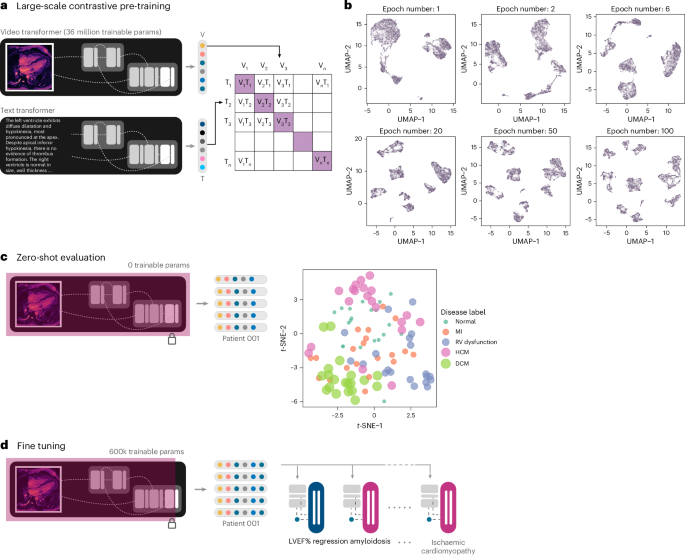
We built on previous attempts at learning visual representations using naturally occurring pairing of 2D medical imaging and textual data, extending these concepts to the spatiotemporal video-like nature of cardiac MRI scans^{14,15,16,17,19,20}. Two parallel encoders were trained: one for processing the MRI cine sequences and the other for processing the subsampled text from paired radiology reports. Self-supervised transformer networks in particular have shown superior performance on downstream tasks compared to traditional supervised techniques^76,81,82. We used an implementation of mViT with Kinetics-400-initialized weights for the vision encoder, and a pre-trained BERT model for the text report encoder. Specifically, we utilized weights from BERT pre-trained on abstracts of biomedical publications on PubMed with a custom vocabulary⁷⁹. Data from 8,513 patients (9,427 scans and paired reports) were used for training, and a separate set from 4,194 patients (4,646 scans and paired reports) were used for validation.

We employed randomized sequential data augmentation schemes (AugMix) to stochastically sample and layer a series of chained transformations including but not limited to resizing, solarization, shear, translate and random rotation of videos in the spatial dimensions, all while preserving the same augmentations along the temporal dimension for temporal consistency⁸³. Uniform temporal subsampling greatly improved downstream performance and generalizability. We augmented the radiology reports by randomly sampling five sentences from the entire report for each scan per training step. The output of each encoder was passed through a one-layer linear projection head to yield a pair of 512-dimensional embeddings. These low-dimensional, 512-dimensional embeddings are a compressed numeric representation of the information contained within the input MRI scan and paired text report.

Previous work has also shown the importance of large batch sizes for effective contrastive representation learning⁸¹. To study this, we pre-trained models with a batch size of 16, 32 and 128 video–text pairs. For the UK BioBank LVEF prediction task, we found that fine tuning from the larger-batch-size pre-trained models led to improved downstream results (Supplementary Fig. 2). While computational budgets did not allow for an extensive hyperparameter search with the larger batch sizes, we note that the downstream benefits did not appear to be clinically significant for this specific task. Nonetheless, this remains an area for additional future exploration.

Vision-only self-supervised methods would be challenging to incorporate where scans from multiple visually distinct view planes exist for the same patient. We focused our efforts on text-to-video approaches given the success with text supervised visual representation learning across radiology and action recognition^14,16,84,85. We considered approaches such as Contrastive Language-Image Pre-Training (CLIP); however, these are limited by a short context length suitable for captions rather than the larger, mostly unstructured paragraphs that are typical of cardiac MRI reports⁸⁵. Similar to the work of ref. ¹⁶, we elected to use an asymmetric bidirectional implementation of the InfoNCE loss to maximize mutual information between each MRI video–text report pair^16,22. The contrastive losses used are essentially log-loss of an n-way classifier to predict the correct pair of MRI scan and report (where n = batch size). The first loss function is a video-to-text contrastive loss for the ith pair, where v_i represents a video embedding and u_i represents a text embedding of the ith video–text pair. N here represents the number of video–text pairs in a total batch being evaluated.

The second loss function is a similarly structured text-to-video contrastive loss. The tunable temperature parameter \(\left({\tau }\right)\) controls the strength of penalties on hard negative pairs sampled during training⁸⁶.

The final loss was defined as a weighted combination of the two losses averaged over all positive video–text pairs in each batch of data. The scalar weight is given by λ.

We additionally implemented a ‘flooding’ regularization technique to prevent the training loss (\({\mathscr{L}}\)) to approach zero⁸⁷. We set the flood level (scalar value given by b) to a training loss of 0.05 to allow for better generalization. The final loss (\(\widetilde{{\mathscr{L}}}\)) is thus given by:

The specific pre-trained weights and vocabulary used for initializing the text encoder, batch size, augmentation scheme, InfoNCE temperature parameter and flood regularization were critical for model convergence⁸⁸. The final model was pre-trained with a batch size of 32 per GPU, for 600 epochs. The first 6 layers of the BERT text encoder was frozen, and the entire network was trained with a learning rate of 4.8 × 10⁻⁵ using the AdamW optimizer with weight decay set to 1 × 10⁻⁶ and eps set to 1 × 10⁻⁸. We decayed the learning rate by a factor of 0.1 at 300 epochs. Checkpoints were saved every 10 epochs during the pre-training process and the last checkpoint was used for fine tuning on downstream clinical tasks. The total time taken for pre-training was 13 days and 14 h (4 × 80 GB Nvidia A100 GPUs). The ability of the vision transformer encoder to cluster different disease conditions without any additional explicit supervised training was visualized using the uniform manifold approximation and projection (UMAP) algorithm initialized using default values⁸⁹.

Multi-instance self-attention and downstream evaluation

A gated multiview self-attention network was trained to assign an attention value (a_k) to each MRI view embedding produced by the main vision encoder^13,31. For each embedding within a bag of k embeddings, a high score after softmax activation (near 1) indicates that a particular MRI view plane is highly informative for the downstream diagnostic task. Conversely, a low score (near 0) indicates that the MRI view plane has little to no diagnostic value. For classification tasks, each input embedding was additionally passed through a LayerNorm function before a forward pass into the self-attention blocks (Supplementary Fig. 6)⁹⁰ (w^T, attention scoring vector; V, view level weight parameters; U, view level weight parameters; h_j, low-dimensional embeddings; ⊙, element-wise product; tanh, tanH activation function; sigm, sigmoid activation function; N, total number of MRI view embeddings for a particular study).

We made use of an attention pooling mechanism to average the embeddings from all MRI views weighted by their predicted attention scores, to return a single 512-dimensional embedding. This embedding can be treated as a ‘feature representation’ of the entire MRI study for a specific downstream task of interest. For each downstream classification task of interest, we used a binary classification head with a sigmoid activation function, as disease labels are usually not mutually exclusive in the setting of cardiovascular disorders. For downstream tasks that involve regression of a numeric variable, we replaced the binary classification head with a single output neuron with a linear activation function.

LVEF regression task

We examined two modes of training for LVEF% prediction: (1) ‘fine tuning’ where the last linear layer of the vision encoder and the classifier head are trainable and (2) ‘transfer learning’ where the vision encoder, linear layer and classifier heads are all trainable. ‘Fine tuning’ allows for some degree of flexibility in the way embeddings are generated but keeps the vision encoder frozen to make use of the learned representations. With the system set to ‘transfer learning’, the network begins from the learned representations; however, since the entire network is unfrozen, it is possible to ‘overwrite’ these parameters with each new update of the training process. For these experiments, we initialized the vision encoder with the contrastive pre-trained weights (ours) or Kinetics-400 weights (baseline), onto which we attached the regression head as described above.

We fine tuned our pre-trained checkpoints with 32-bit precision using the AdamW optimizer, with a learning rate set to 1 × 10⁻⁴ and default value of 0.01 for weight decay. We explored different augmentation schemes and achieved superior validation performance with AugMix on restricted hyperparameter sweeps with 10% of the training data⁸³. For all experiments involving fine tuning with subsets of available data, we used a manual seed value for random subsampling to ensure reproducibility of results. We made use of all available 4CH, 2CH, 3CH and a random subsample of 50% of SAX views per study, with no manual screening for quality control. We elected to train our regression models with a Huber loss function, and we used mean squared errors and mean absolute errors as performance metrics⁹¹. We additionally calculated the AUROC for diagnosing heart failure on the basis of an LVEF cut-off of 40%. We trained models for a maximum of 100,000 steps on GPUs with at least 16 GB of VRAM each. For experiments described in Fig. 3a,d, configuration files were generated for each experimental setup and were trained in parallel across numerous GPUs on Stanford Sherlock.

Disease classification task

We define both ‘fine tuning’ and ‘transfer learning’ as above, and used the same network architecture initialized with Kinetics-400 weights as our baseline. We fine tuned our pre-trained checkpoints with the same overall settings as described above for the regression tasks, except for the use of a weight decay value of 5 × 10⁻⁴ and the addition of a LayerNorm function for the embeddings before a forward pass through the multi-instance self-attention modules to aid with convergence. We empirically used AugMix for our data augmentation strategy, given the successes noted above. We made use of all available 4CH, 2CH, 3CH and SAX views per study with no quality control or screening. We utilized a binary cross-entropy loss function with a sigmoid activation weighted by a scalar multiplier equal to the proportion of positive vs negative classes for each disease (calculated using the internal training set prevalences). We used the AUROC as a performance metric, given the considerable class imbalance of positive and negative classes⁹². For each disease label of interest, we trained models for 24 epochs on GPUs with at least 24 GB of VRAM. For experiments described in Fig. 4a,b, configuration files were generated for each experimental setup and were trained in parallel across numerous GPUs on Stanford Sherlock. External test data were evaluated on the Penn CBICA cluster on a single Nvidia A40 GPU with 40 GB VRAM, and on the PARCC Betty cluster on a single Nvidia Blackwell B200 GPU with 180 GB VRAM. In addition to the losses and metrics, we stored predicted probabilities and relative self-attention scores for each view for downstream processing and statistical analyses.

Statistical analyses

We used the torchmetrics (v.1.0.1) package to calculate MSE and MAE for regression tasks, and AUROC values for classification tasks within the training and validation loops. We additionally manually calculated AUROCs as empirical curves in the sensitivity and specificity space, computed from predicted probabilities generated by our models⁹³. To compare the performance of fine-tuned classifier models (that is, contrastive pre-trained vs baseline), we calculated non-parametric confidence intervals on the AUROC using DeLong’s method (paired)⁹⁴, following which P values were computed for the mean difference between AUROC curves. Additional analyses were performed to calculate the accuracy for each diagnostic label at different thresholds (optimizing for Youden’s statistic, a sensitivity of 0.90 or a specificity of 0.90). Differences between predicted LVEF% values and ground truth were assessed using Bland–Altman plots. Statistical analyses were performed and graphs were plotted using R (v.4.1.0); major packages used included pROC (v.1.17.0), ggplot2 (3.3.5) and blandr (0.5.1). The online test-set leaderboard webapp was created using shiny (1.8.1).

Attention visualizations

For every input scan, we output the raw self-attention tensors from each head of each layer of the MRI vision encoder during evaluation and processed them to yield 65 separate attention heat maps. As described earlier, the spatiotemporal resolution was reduced with each successive stage in the mViT architecture; the self-attention tensors were reduced from an initial spatiotemporal resolution of 8 × 56 × 56 at the first layer, to 8 × 7 × 7 at the last few layers. We kept only the attention values from the output patches for the purposes of visualization, and spatiotemporally interpolated these tensors back to a size of 16 × 224 × 224 via nearest-neighbour resampling. These arrays were exported to mp4 files using imageio and the ffmpeg library (Supplementary Figs. 17 and 18). Aside from the self-attention heat maps for each input video, we also computed the raw self-attention values from the multi-instance classifier head for relevant downstream tasks. After each scan was passed through the vision encoder, the resultant embedding was assigned a leaned raw self-attention score within the multi-instance self-attention modules. We calculated the relative differences in self-attention scores across different view planes for each disease label. These relative self-attention values were visualized as 2D heat maps as shown in Fig. 4c. The multi-instance classifier head self-attention scores showed that the network learns to differentially prioritize view planes for different clinical tasks.

Reporting summary

Further information on research design is available in the Nature Portfolio Reporting Summary linked to this article.